7.11 EMP_mutate

​ The EMP_mutate module is highly versatile, allowing transformations not only based on assay, rowdata, and coldata of a dataset, but also on the results of data analysis. To help users better understand its usage, the basic parameters of the module are described below:

• obj ： Specifies the input object, which can be an MAE or EMPT.
• experiment ： Specifies the name of the omics assay to analyze (character).
• ... ：Inherited from the dplyr::mutate() function, supporting a variety of data transformations.
• .by : Inherited from dplyr::mutate(); equivalent to performing group_by() before the transformation.
• .before : Inherited from dplyr::mutate(); sets the position of the new column to be placed before a specified column.
• .after : Inherited from dplyr::mutate(); sets the position of the new column to be placed after a specified column.
• mutate_by: Specifies whether the transformation is applied by sample or by feature.
• location：Defines where the new column is created — in assay, rowdata, or coldata.
• action: A character string selecting between "colwise" and "rowwise", indicating whether the operation should be performed column-wise or row-wise.
• keep_result: If the input is TRUE, it means to keep all analysis results, regardless of how samples and features change. If the input is a name, it means to keep the corresponding analysis results.

7.11.1 Mutate for the MultiAssayExperiment

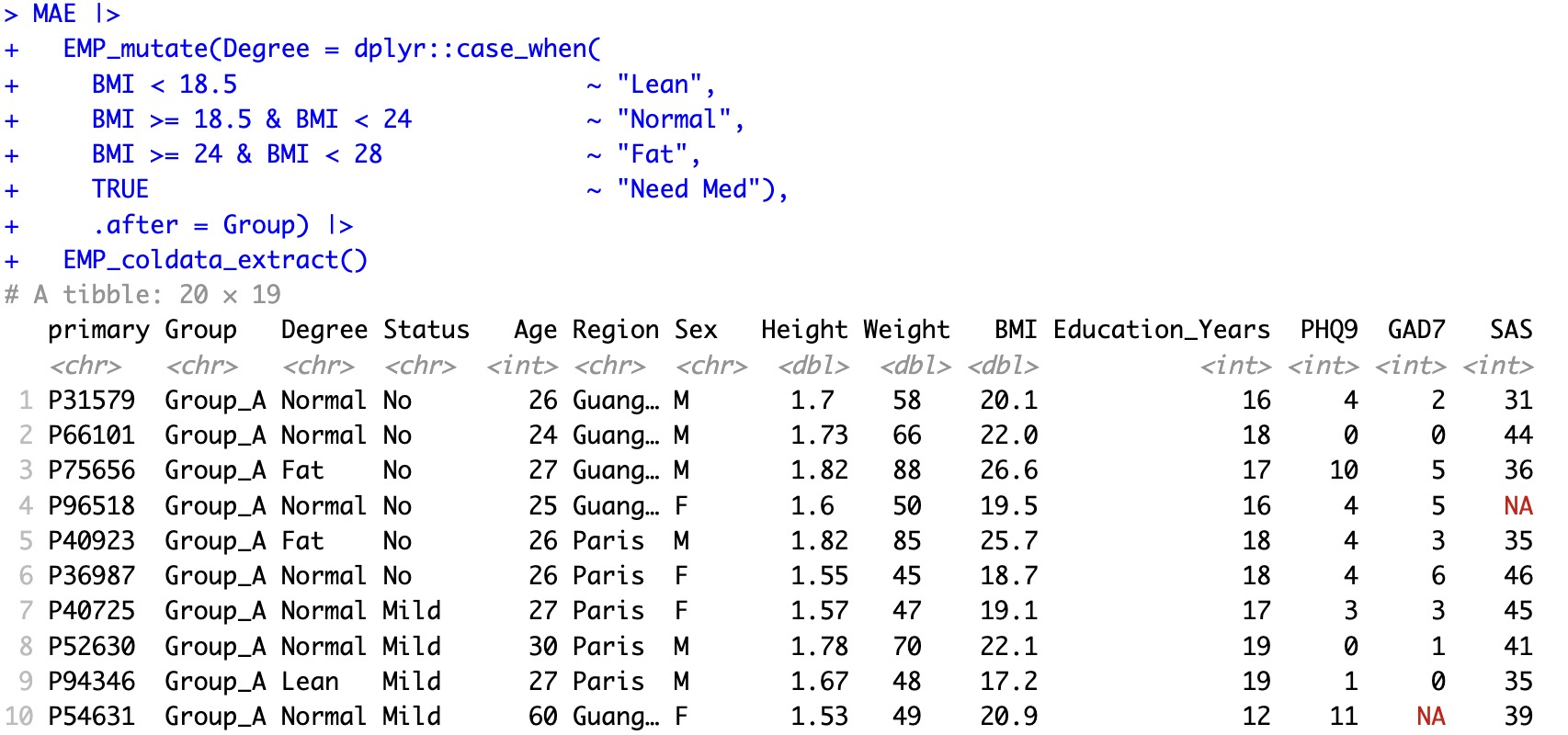
🏷️Example： Create a new group.

MAE |>
  EMP_mutate(Degree = dplyr::case_when(
    BMI < 18.5                        ~ "Lean",
    BMI >= 18.5 & BMI < 24            ~ "Normal",
    BMI >= 24 & BMI < 28              ~ "Fat",
    TRUE                              ~ "Need Med"),
    .after = Group)

After mutating, users can use the module EMP_coldata_extract to observe the result.

MAE |>
  EMP_mutate(Degree = dplyr::case_when(
    BMI < 18.5                        ~ "Lean",
    BMI >= 18.5 & BMI < 24            ~ "Normal",
    BMI >= 24 & BMI < 28              ~ "Fat",
    TRUE                              ~ "Need Med"),
    .after = Group) |>
  EMP_coldata_extract()

7.11.2 Mutate for the signle omics data

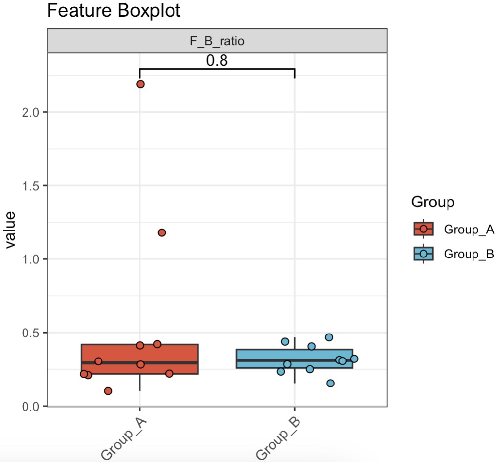
🏷️Example1： Compute the Firmicutes-to-Bacteroidetes ratio.

MAE |>
  EMP_assay_extract('taxonomy') |>
  EMP_collapse(collapse_by = 'row',estimate_group = 'Phylum') |>
  EMP_mutate(F_B_ratio = Firmicutes/Bacteroidetes,
             .by = primary,.before = 2,
             mutate_by = 'sample',location ='assay') |>
  EMP_filter(filterFeature = 'F_B_ratio') |>
  EMP_boxplot(estimate_group='Group')

🏷️Example2：This process integrates results from multiple differential analysis algorithms and adds annotation information to the features.

MAE |>
  EMP_assay_extract('host_gene') |>
  EMP_diff_analysis(method = 'wilcox.test',estimate_group = 'Group') |>
  EMP_mutate(wilcox = pvalue,
             wilcox_fdr = fdr,
             mutate_by = 'feature',location ='rowdata') |>
  EMP_diff_analysis(method = 'DESeq2',.formula = ~Group) |>
  EMP_mutate(DESeq2 = pvalue,
             DESeq2_fdr = fdr,
             mutate_by = 'feature',location ='rowdata')

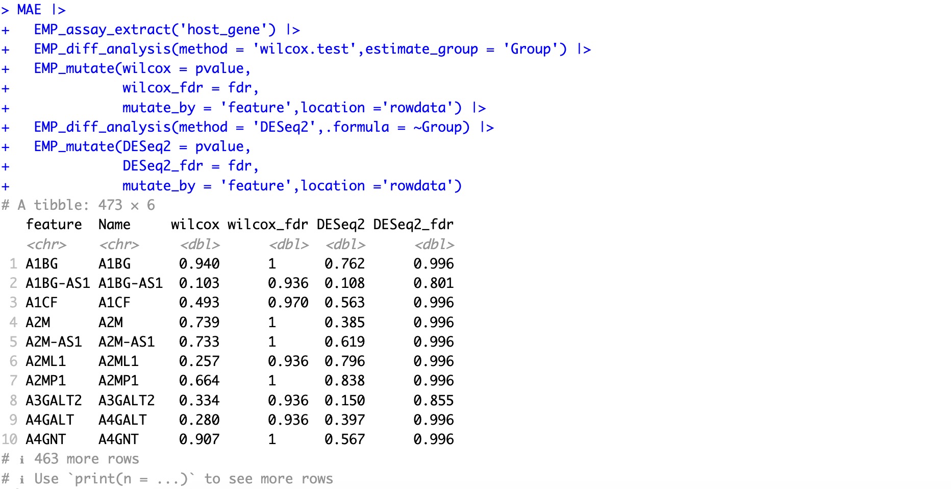
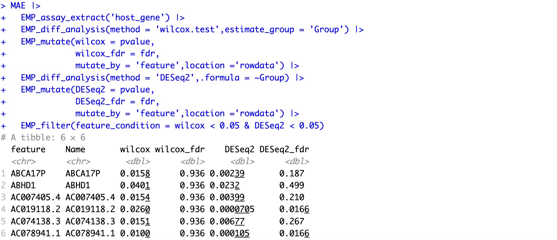
This allows us to identify feature genes that are significant in both differential analysis methods.

MAE |>
  EMP_assay_extract('host_gene') |>
  EMP_diff_analysis(method = 'wilcox.test',estimate_group = 'Group') |>
  EMP_mutate(wilcox = pvalue,
             wilcox_fdr = fdr,
             mutate_by = 'feature',location ='rowdata') |>
  EMP_diff_analysis(method = 'DESeq2',.formula = ~Group) |>
  EMP_mutate(DESeq2 = pvalue,
             DESeq2_fdr = fdr,
             mutate_by = 'feature',location ='rowdata') |>
  EMP_filter(feature_condition = wilcox < 0.05 & DESeq2 < 0.05)

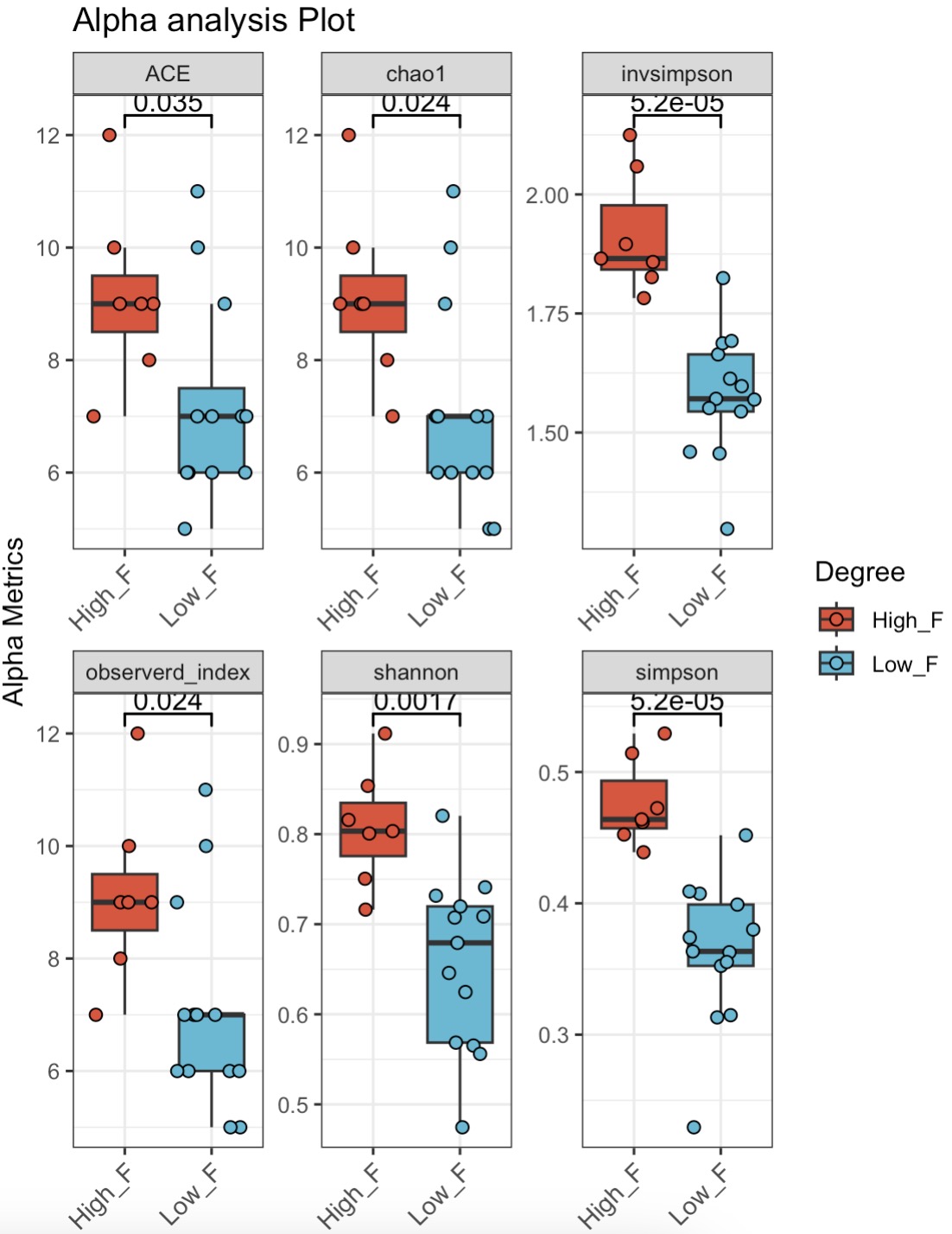
🏷️Example3：Grouped by Firmicutes abundance levels and compared for alpha diversity.

MAE |>
  EMP_assay_extract('taxonomy') |>
  EMP_collapse(collapse_by = 'row',estimate_group = 'Phylum') |>
  EMP_mutate(Degree = dplyr::case_when(
    Firmicutes >= mean(Firmicutes)     ~ "High_F",
    Firmicutes <  mean(Firmicutes)     ~ "Low_F"),
   .after = Group) |>
  EMP_alpha_analysis() |>
  EMP_boxplot(estimate_group='Degree')